The perceptron: a model that decides
From calculation to decision
Neural networks represent the influence of inputs through weights. Adjusting those weights to fit data lets a model learn relationships between inputs and outcomes, then calculate results for new inputs. It might predict a house price from its size, location, and age, or use information in an image to distinguish cats from dogs.
But a weighted sum alone only produces a number. It does not, by itself, specify how to turn that number into a category or a yes-or-no decision.
We want models that use data to perform some of the judgments people make. How can a calculation become a decision? An early neural network model that addressed this question was the perceptron.
Setting a decision threshold
A perceptron is a simple neural network model that takes several inputs and produces one output. It resembles an artificial neuron, with the added rule that its calculation selects between two possible outcomes.
It first multiplies each input by its weight and adds the products. We can think of this weighted sum as a score combining the evidence from the inputs. The score still needs to be turned into a decision.
A value called the bias adjusts the decision threshold. It is added to the weighted sum. Increasing it makes the positive outcome easier to select for the same inputs; decreasing it means a larger weighted sum may be needed.
The perceptron bases its decision on this weighted sum plus bias.
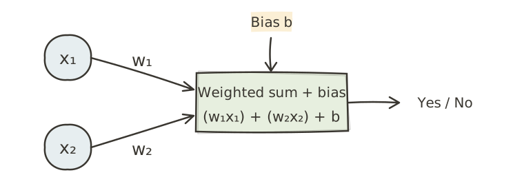
Let’s build a very simple spam classifier. It will use a few clues in an email to decide whether the message is spam.
The model combines the weighted clues with a bias to produce a score. We will classify the email as spam if the score is greater than 0, and not spam if it is 0 or less.
We need to choose our clues first. Here, we will check whether the message contains the word “free” and whether its sender is unknown. Set x₁ to 1 when “free” is present and 0 otherwise. Set x₂ to 1 for an unknown sender and 0 for a known sender.
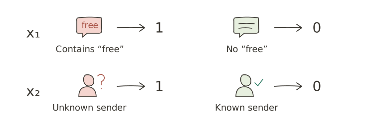
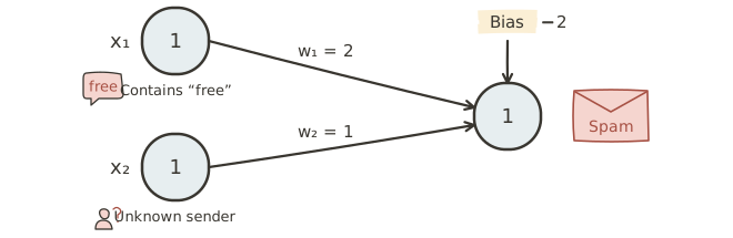
For now, we will treat “free” as the stronger clue: give x₁ a weight of 2 and x₂ a weight of 1. Set the bias to -2. We will see what that does through the calculations.
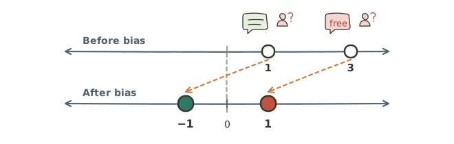
Suppose an email contains “free” and comes from an unknown sender. Its score is (1 × 2) + (1 × 1) - 2 = 1. Since the score is greater than 0, the model classifies it as spam.
Now suppose the sender is unknown, but the message does not contain “free.” The score is (0 × 2) + (1 × 1) - 2 = -1. Since it is not greater than 0, the model classifies this message as not spam.
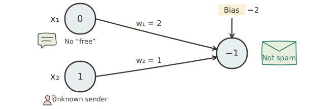
Without a bias, these examples would have scores of 1 and 3. Both would exceed 0, so both would be classified as spam.
Adding the bias -2 changes those scores to -1 and 1. Now only an email with both clues is classified as spam. In this example, a bias of -2 means that the weighted sum must exceed 2. Changing the bias can change the decision even when the inputs and weights stay the same.
Turning the score into an output
So far, we have checked the score ourselves. The perceptron can also perform that final step. An activation function transforms the score into the output.
For our example, the function compares the score with 0. A score greater than 0, such as 1, produces output 1. A score of 0 or less, such as -1, produces output 0.
We can draw this rule as a decision tree:
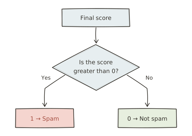
This gives us an unambiguous decision, but it also creates a sudden jump. Moving the score from -0.01 to 0.01 changes the output from 0 to 1, even though the scores are almost identical.
The two possible outputs also hide how far the score is from the threshold. Scores of 0.01 and 100 both produce 1.
More complex models often benefit from activation functions that respond more gradually or produce a wider range of values. Different functions transform their inputs in different ways.
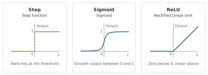
The horizontal axis, z, represents the score. Our spam example uses a step function: output 1 when z > 0, otherwise 0.
Other choices include the sigmoid function, which changes smoothly, and ReLU, which outputs 0 for nonpositive inputs and leaves positive inputs unchanged. The appropriate function depends on the problem and training method. ReLU and its variants are common in deep learning because their calculations are simple and they can support effective training.
Putting the pieces together, the model first calculates a weighted sum, then adds the bias, then applies the activation function.
For two inputs, we can write the full calculation as y = activation(w₁x₁ + w₂x₂ + b):
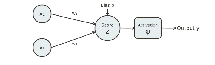
Here, z is the weighted sum plus bias, and φ (phi) denotes the activation function. It transforms the score z into the output y according to its rule.
Learning from mistakes
We chose w₁ = 2, w₂ = 1, and b = -2 ourselves. We specified the importance of each clue and the threshold for calling an email spam. Up to this point, we have built a hand-written rule rather than learned one from data.
In machine learning, we do not give the model the final weights and bias as answers. Instead, we show it examples labeled as spam or not spam and let a learning procedure adjust the values.
The basic idea is to predict using the current weights and bias, then compare the prediction with the correct answer. When the prediction is wrong, adjust the parameters. Repeating this process aims to reduce errors.
The learning objective
A loss expresses prediction error as a number. A loss function calculates that number from predictions and targets. Different tasks call for different loss functions.
One simple example is squared error. If y is the target and ŷ is the prediction:

Squaring the difference makes the loss nonnegative and makes larger errors more costly. For a target of 1, a prediction of 0.8 gives a loss of 0.2² = 0.04. A prediction of 0.2 gives a loss of 0.8² = 0.64.
Although the loss function varies, the broad training objective is the same: adjust the weights and bias to reduce error. Loss gives us a numerical way to assess progress.
The squared-error example illustrates loss in general. The classic perceptron uses a mistake-driven update rule, which we will illustrate next; it does not directly differentiate squared error through the step function.
The learning process
Suppose we collect 100 emails for each combination of the two clues. Messages with both “free” and an unknown sender are most often spam; messages with neither clue are least often spam.
Contains “free” (x₁) |
Unknown sender (x₂) |
Spam emails | Spam rate |
|---|---|---|---|
| 1 | 1 | 91 / 100 | 91% |
| 1 | 0 | 42 / 100 | 42% |
| 0 | 1 | 18 / 100 | 18% |
| 0 | 0 | 3 / 100 | 3% |
We do not feed these percentages into the perceptron. We feed individual emails, predict from their clues, and compare the prediction with each email’s label. The examples reveal that the two clues together are strongly associated with spam.
Let’s walk through some updates. Start with w₁ = 0, w₂ = 0, and b = 0.
First, take an actual spam email containing “free” from an unknown sender. Its score is 0, so our step function predicts not spam. The prediction is wrong.
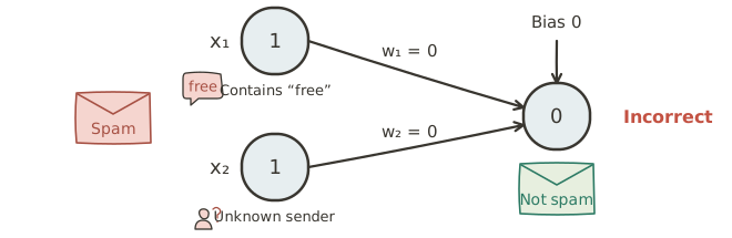
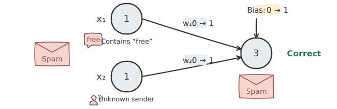
We need to increase the score. Both inputs are 1, so increasing either weight increases it. Increasing the bias also increases it, regardless of the input values.
For a simple demonstration, increase w₁, w₂, and b by 1 each. The score becomes (1 × 1) + (1 × 1) + 1 = 3. The model now correctly predicts spam for this example.
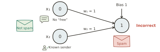
Next, take a legitimate email with neither clue. Both inputs are 0, so the weighted sum is 0. Adding the current bias of 1 gives a score of 1, incorrectly predicting spam.
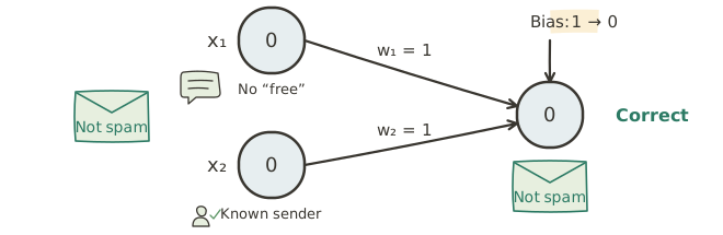
To lower the score, reduce the bias by 1, bringing it to 0. The score becomes 0, so the model now correctly predicts not spam. Because both inputs are 0, changing their weights would not change the score for this example.
Repeated updates can find useful combinations of weights and bias, such as the illustrative w₁ = 2, w₂ = 1, b = -2 rule we started with. The exact values depend on the data and update process. Our table contains conflicting labels for identical inputs, so no classifier using only these two clues can classify every email correctly.
Settings that affect learning
By updating values to correct mistakes, the perceptron searches for weights and a bias that fit the data.
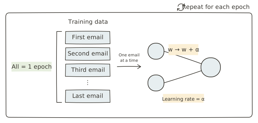
One pass through all training examples is called an epoch. Training often involves several epochs, during which we can monitor errors. We might stop when all examples are classified correctly, when progress stalls, or when we reach a chosen number of epochs. Perfect classification is only possible when the data and model allow it.
We used changes of 1 to keep the arithmetic simple. A learning rate controls the size of updates. In our binary-input example, a learning rate of 0.1 could produce updates of 0.1 to active weights and the bias, while 0.5 could produce updates of 0.5. More generally, the learning rate scales an update that also depends on the training rule and data.
The learning rate can affect training speed and stability. In many training methods, an excessively large rate can overshoot useful values, while a very small one can make progress slow.
In chapter 1, we used the illustrative function f(x) = ax + b and called values such as a and b parameters. The perceptron’s weights and bias are parameters too: training adjusts them.
OpenAI’s GPT-3, introduced in 2020, had 175 billion parameters. That gives a sense of how many values a large language model can adjust during training. Some model developers do not publish parameter counts, and parameter count alone does not determine a model’s capabilities.
Is the learning rate a parameter too? It is usually a setting we choose to control training, rather than a value learned in the same way as the weights and bias. Such settings are called hyperparameters. They govern how learning takes place.
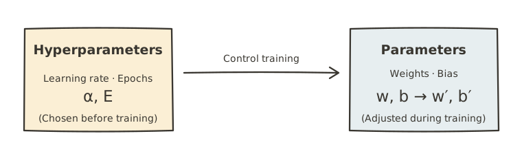
Hyperparameters can strongly affect training and the final result. Trying different settings and comparing their performance is called hyperparameter tuning.
There is more than one solution
A useful decision rule does not necessarily have a unique set of parameters. For example, doubling w₁ = 2, w₂ = 1, and b = -2 gives w₁ = 4, w₂ = 2, and b = -4, with the same classification results.
The scores double, but the step function only checks whether they exceed 0. A score of 1 or 2 produces the same output. Different parameter values can therefore lead to the same decisions.
What matters is how well the model works on new examples. Applying what it has learned to unseen data is called generalization. We want a model that does more than fit its training examples.
To assess this, we set aside validation data before training and do not use it to update the weights. We compare predictions on those examples with their labels to evaluate performance and help choose a model or hyperparameter settings that work beyond the training data.
Exercises
Decide whether each statement is True or False.
- The bias adjusts the threshold at which a perceptron selects an outcome.
- A lower loss means predictions are closer to the targets under the chosen loss function.
- One epoch is one pass through the training dataset.
- A larger learning rate always makes training more stable.
- Weights and bias are hyperparameters chosen by the person training the model.
Answers and explanations
- True — Adding the bias shifts the score used for the decision.
- True — Loss measures prediction error according to the chosen function.
- True — An epoch uses the full training dataset once.
- False — A rate that is too large can make updates overshoot in many training methods.
- False — Weights and bias are learned parameters. Settings such as learning rate are hyperparameters.