Multilayer networks: working backward

The limits of a single layer

A network that calculates its output directly from the input layer, like our perceptron, is called a single-layer neural network. The input layer only passes data onward, so we do not count it as a computational layer. The output layer is the only layer performing calculations.

It multiplies inputs by weights, adds them together, and makes a decision from the score. Whether there are two inputs or hundreds, it makes one judgment: “Does the combined score pass the threshold?”

Each input contributes independently to that score. Once the weight for “free” is set, its contribution is the same whether or not the sender is unknown. This works for patterns that can be recognized by adding up evidence, but it has limits when the relationship between conditions matters.

Imagine a cooperative game in which two players independently choose left or right. They win if they choose the same direction and lose if their choices differ.

Both-left and both-right must produce a win, while mixed choices must produce a loss. A single-layer perceptron cannot express this rule, no matter how we choose its weights and bias. Let’s see why.

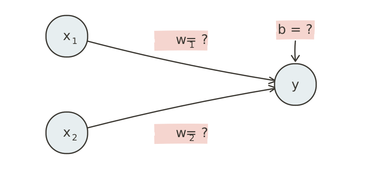
Encode left as 0 and right as 1. For this proof, let a score of 0 or greater mean a win.

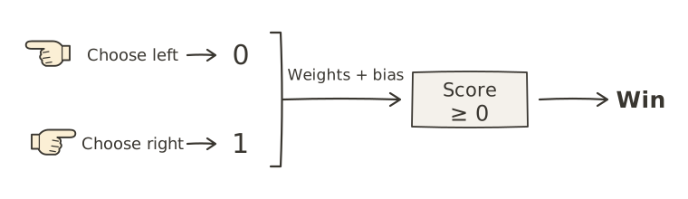
When both players choose left (0), both weighted inputs vanish. The bias alone must produce a winning score, so ① b ≥ 0.

When only one player chooses right, the score is either w₁ + b or w₂ + b. Both must be negative, so ② w₁ < −b and w₂ < −b.

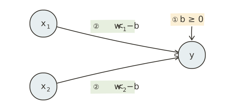
When both choose right (1), the score is w₁ + w₂ + b.

From ②, w₁ + w₂ < −2b. Adding the bias gives w₁ + w₂ + b < −b.

Since ① requires b ≥ 0, we get ③ w₁ + w₂ + b < −b ≤ 0.

But both-right must also win, which requires ④ w₁ + w₂ + b ≥ 0.

Conditions ③ and ④ contradict each other. No combination of weights and bias can satisfy this rule.

Solving it by adding layers

This is a limitation of the model’s structure, not a lack of training. Training it longer cannot make the rule representable.

We can overcome this by stacking layers of units. Units in the first layer detect different patterns in the inputs and pass their results onward. The next layer combines those results as new inputs. With nonlinear activation functions, this structure can represent more complex relationships.

A network of this kind is called a multilayer perceptron (MLP).

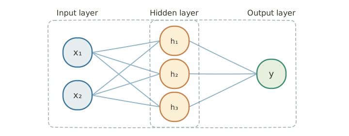
Each unit calculates a weighted sum, adds a bias, and applies an activation function. The diagram leaves those details out to emphasize the connections.

A layer between the input and output layers is called a hidden layer. Its neurons, such as h₁, h₂, and h₃, calculate intermediate results.

“Hidden” means that these values are created inside the model, rather than supplied as inputs or observed as final outputs.

A multilayer network can represent our cooperative game. We want the players to win when their directions match.

The first hidden neuron, h₁, can detect “both chose left.” The second, h₂, can detect “both chose right.” The output neuron then reports a win if either hidden neuron is active.

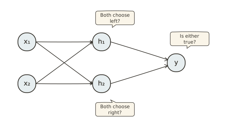
Matching directions now produce a win, while mixed directions produce a loss. Rather than make one judgment directly from the raw inputs, the network detects smaller patterns in the hidden layer and combines them in the output layer.

Let’s choose weights and biases that implement this rule. For x₁ = 1 and x₂ = 1, both players choose right:

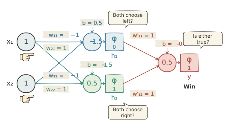
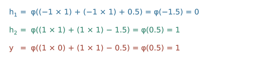
This worked example uses the step activation function φ from chapter 3: output 1 when the score is greater than 0, otherwise output 0. The chosen scores are away from the threshold, so this convention gives the intended game results.

Why learning becomes harder

For a single-layer perceptron, we can directly identify which inputs contributed to a mistake. If it misses a spam email, we adjust the weights connected to that email’s clues in the appropriate direction.

Training a multilayer network is more complicated. The data gives us the correct final answer y, but not the desired values of hidden neurons h₁ and h₂. When the final prediction is wrong, which weights should change, by how much, and in which direction? With more layers, tracing the error back to the many earlier weights becomes increasingly difficult.

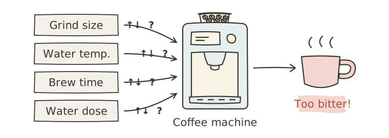
Think of an automatic coffee machine. If the coffee tastes too bitter, changing the grind size, water temperature, brew time, or amount of water can affect the result. But “too bitter” alone does not tell you which setting to change or by how much. Similarly, knowing that a network’s prediction is wrong does not immediately reveal how each weight should be adjusted.

The chain rule

Fortunately, there is a way to calculate these relationships. The chain rule connects derivatives across successive calculations. It lets us work backward from the loss to determine how each weight affects it.

If derivatives sound unfamiliar, think of a derivative as describing how quickly one quantity changes as another changes.

A moving car changes position over time. Looking at its change in position over a very short time interval leads to its instantaneous speed. More precisely, the derivative of position gives velocity. If position is x and time is t, we write dx/dt for that rate of change.

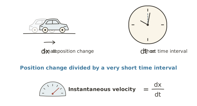
For a network, we want to know how changing a weight w affects the loss L. We can write this informally as dL/dw. It tells us the direction and steepness of the change in loss as the weight changes slightly. We can use that information to adjust the weight toward a lower loss.

Consider one path by which a weight affects the result. It changes a weighted sum z, which passes through an activation function to produce a hidden value h⁽¹⁾. Its influence continues through later hidden layers to h⁽ᵏ⁾, then the output y, and finally the loss L. The parenthesized superscripts identify the hidden layers.

A weight’s effect passes through several stages, so we need to account for the changes at each stage. The chain rule’s key idea is to multiply the rates of change along a path to obtain its overall effect.

Individual stages, such as a weighted sum or activation function, have relatively simple formulas. Their derivatives are therefore easier to calculate than the derivative of the entire network at once.

For a path with one hidden layer:

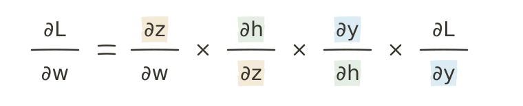
The left side describes how the loss changes with the weight. The right side follows the chain of effects through z, h, y, and L. When a value influences the loss through several paths, we add the contributions from those paths.

Earlier we used d for derivatives. Neural network calculations usually use ∂, the symbol for a partial derivative. When a result depends on many variables, a partial derivative describes its sensitivity to one variable while treating the other independent variables as fixed. Since many weights and biases determine the loss, we use partial derivatives to study their effects individually.

The hard step functions in the game example demonstrate what the network can represent. For practical backpropagation, we normally use activations with useful derivatives, such as sigmoid or ReLU, rather than differentiating through a hard threshold.

Working backward

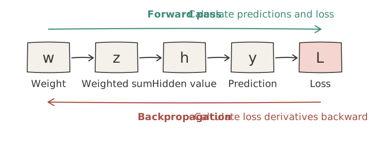
Calculating a prediction from the input through the hidden and output layers is called forward propagation, or the forward pass. Comparing that prediction with the target gives a loss.

To reduce the loss, we need derivatives with respect to the network’s weights and biases. The chain rule provides them.

Many weights share parts of the computation leading to the loss. If we calculated every derivative independently from scratch, we would repeat the same work many times. Instead, we can reverse direction: start at the loss and work backward through the output and hidden layers. Derivatives calculated for later stages can be reused at earlier stages.

This efficient backward application of the chain rule is called backpropagation.

Backpropagation calculates derivatives; it does not update the weights itself. An update rule uses those derivatives to adjust the parameters. Reusing calculations makes it practical to find the influence of many interconnected weights, providing an essential foundation for training deep networks.

Geoffrey Hinton and backpropagation

In 1986, Geoffrey Hinton, David Rumelhart, and Ronald Williams helped popularize training networks with hidden layers using backpropagation. Hinton’s subsequent work on Boltzmann machines and other models also shaped deep learning. In 2024, he shared the Nobel Prize in Physics with John Hopfield for foundational discoveries and inventions enabling machine learning with artificial neural networks.

Image: Xuthoria · CC BY-SA 4.0

Exercises

Decide whether each statement is True or False.

1. A single-layer perceptron can represent every rule involving combinations of conditions.
2. Hidden-layer values are intermediate results created inside the model and passed to the next layer.
3. ReLU outputs 0 for inputs below 0.
4. The chain rule lets us calculate a rate of change through successive stages by multiplying their derivatives along a path.
5. Backpropagation calculates derivatives from the input layer toward the output layer.