Learning in high-dimensional spaces

Vectors in space

We have used many numbers for inputs, weights, biases, and outputs. Numbers with the same role can be grouped: three inputs become [x₁, x₂, x₃], and their weights become [w₁, w₂, w₃]. An ordered collection of numbers treated as one object is a vector.

Each value is a component. A vector with three components is three-dimensional; one with n components is n-dimensional.

Vectors also have a geometric interpretation. Draw one as an arrow, and you can examine its direction, length, and relationship to other vectors.

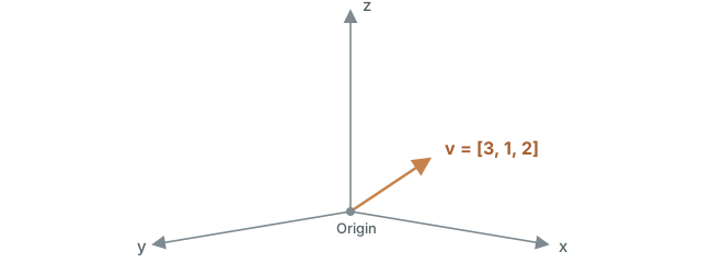
The computer stores numbers and performs operations; it does not need to picture an arrow. But the geometric viewpoint helps us reason about many values together. We can represent a vector as a point or arrow in an n-dimensional space.

We cannot directly visualize four or more dimensions, so diagrams usually simplify the idea to two or three. The mathematical operations still extend to higher dimensions.

Learning and vectors

Weights and biases can also be collected into a parameter vector. Training changes its components, which moves the corresponding point in parameter space. We repeatedly seek positions with lower loss.

Changing the weight vector also changes its dot product with an input vector. A dot product multiplies corresponding components and adds the products. Geometrically, it measures alignment while also accounting for vector lengths. With lengths fixed, similar directions give a larger dot product, perpendicular vectors give 0, and opposing directions give a negative value.

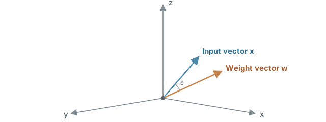
The dot product of an input vector and a weight vector is exactly the weighted sum w₁x₁ + w₂x₂ + w₃x₃.

For a perceptron, it is a score evaluating the input according to the current weights. Changing those weights means changing the criteria used to evaluate the same input. The score, and possibly the final decision, changes.

Training adjusts weights to reduce prediction error. It can make useful input features contribute more effectively and less useful features contribute less. This does not mean that a large weight alone always proves a feature is important: feature scales and other weights matter too.

Finding lower loss

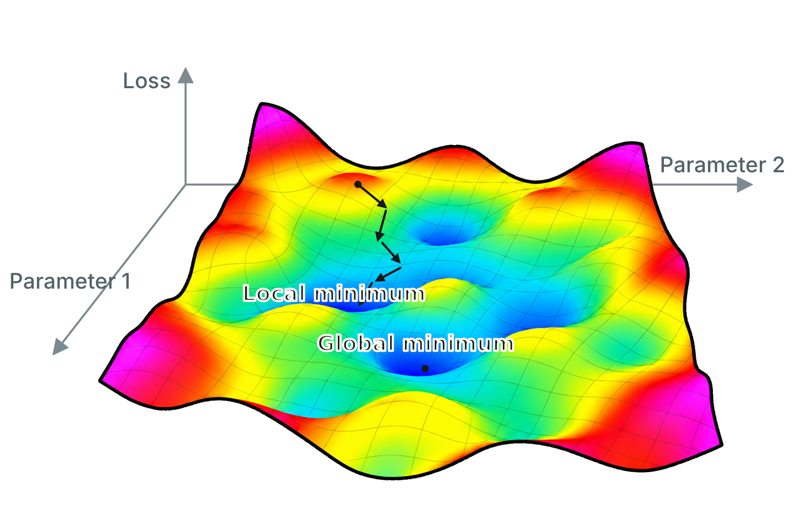
Fix the parameters and evaluate the model on a dataset, and you obtain a loss. We can picture the parameter combination as a location and the loss as its height.

Across different parameter combinations, high-loss regions become hills and low-loss regions become valleys. This picture is called a loss landscape.

Real networks have far more dimensions than we can draw. For illustration, we will pretend there are just two parameters and use a third axis for loss.

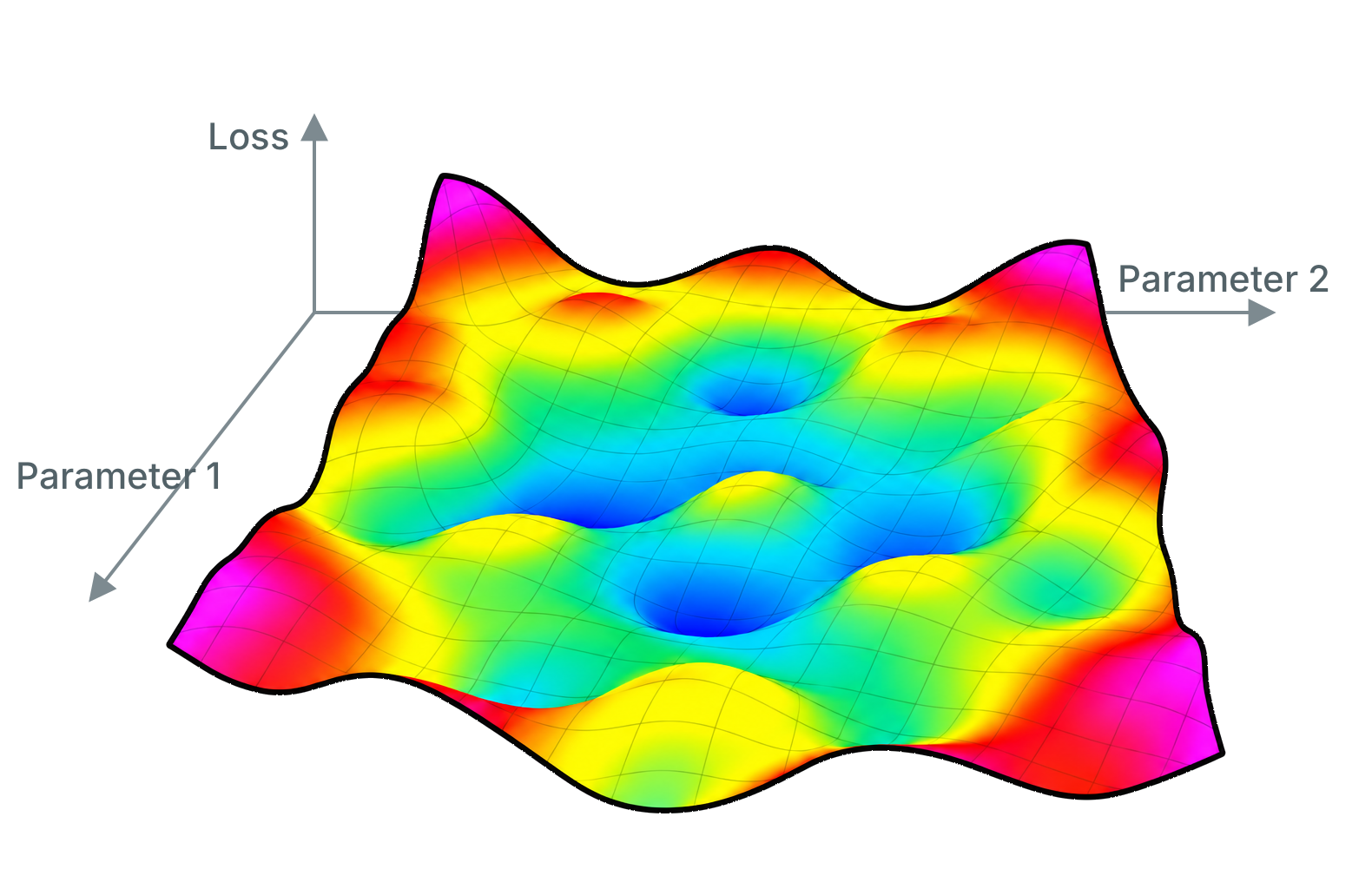
Training does more than evaluate loss: it changes the parameters to find a lower value. Searching for a minimum, or a sufficiently good low-loss region, is optimization.

Finding the steepest descent

Backpropagation gives us loss derivatives for the weights and biases. Collecting them produces a gradient. For w₁, w₂, and b, it is the vector (∂L/∂w₁, ∂L/∂w₂, ∂L/∂b).

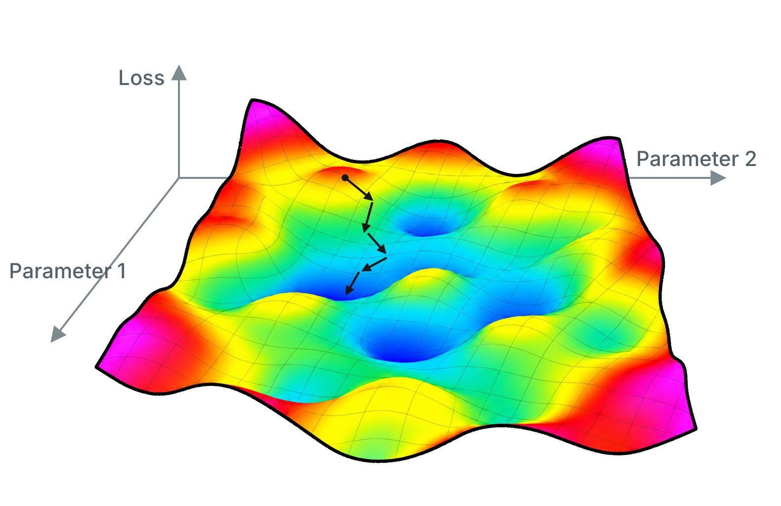
The gradient points in the direction of the steepest local increase in loss. Taking a sufficiently small step in the opposite direction can reduce the loss.

This is gradient descent: inspect the local slope and repeatedly step downhill, rather like finding your way down a mountain by checking the ground beneath your feet.

A loss landscape need not be a single smooth bowl. A valley may be lower than its immediate surroundings without being the lowest point overall. Such a point is a local minimum. The lowest value across the entire space is a global minimum.

Near a local minimum, small movements do not decrease loss. A method driven only by the local gradient can therefore have difficulty reaching a better region if the route first goes uphill. High-dimensional optimization also encounters flat regions and saddle points, so local minima are not its only challenge.

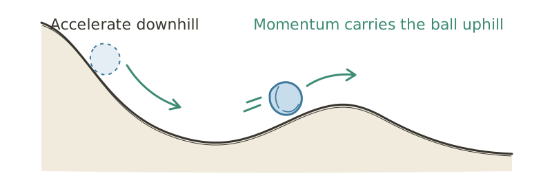
Optimizers extend basic gradient descent to improve speed or stability. Momentum retains part of the previous update direction, somewhat like inertia. A rolling ball can build speed downhill and carry it over a shallow rise. Momentum can produce a similar effect, although it does not guarantee escape from every local minimum.

The Adam (Adaptive Moment Estimation) family combines moving averages of gradients with information about their magnitudes to scale updates for individual parameters. It is widely used in deep learning.

Is the lowest point always best?

We do not necessarily need to reach a global minimum. A nearby local minimum may have almost the same loss, and finding a lower one might not justify the extra computation.

More importantly, minimizing training loss is not the ultimate goal. Generalization—performing well on unseen data—matters.

A solution that closely fits every detail of the training data can perform poorly on new examples. Another solution may have slightly higher training loss but better generalization.

We therefore use held-out validation data to evaluate generalization as well as training loss.

Exercises

Decide whether each statement is True or False.

1. A vector with three components is three-dimensional.
2. A dot product multiplies corresponding components and adds the products.
3. Gradient descent moves parameters in the direction of the gradient.
4. Reaching a local minimum means training has failed.
5. Momentum guarantees escape from every local minimum.